Abstract
Phytoplankton can be bioindicators to assess water quality in freshwater ecosystems. In this study, phytoplankton biomass responses to temperature, sunlight, water body size, and water body connectivity were evaluated to justify their sensitivity as the water quality indicator. 65434 observations from LAGOS-NE were analyzed to show the correlation between phytoplankton biomass and abiotic factors. Increasing temperature, increasing sunlight, increasing lake size showed positive effects and less water body connections showed significantly positive influences on phytoplankton biomass. Also, phytoplankton responses to environmental changes were found to have high possibilities to be associated with N and P conditions in the water. Consequently, their performance can reflect the water quality and the extent of eutrophication of freshwater ecosystems.
Introduction
Sustainable water management is a priority for science and research. Water quality describes the condition of water, usually concerning its suitability for purposes such as drinking or swimming (Diersing & Nancy, 2009). While water quality is traditionally defined based on physical parameters like temperature, salinity, and oxygen. Phytoplankton is a useful bioindicator of water quality because their populations respond quickly to environmental changes (Gharibet.al., 2011) and they are connected to the rest of the ecosystem through their productivity ( Behrenfeld, 2001). Recent studies have already tried this application and proved the feasibility of this method from their results. They suggested that phytoplanktons reflect water quality and the extent of eutrophication through changes in its biomass (Suthers, Rissik, & Richardson, 2019), community structure (Parmar, Rawtani & Agrawal, 2016), patterns of distribution (Amengual-Morro, Niell & Martínez-Taberner, 2012) and the proportion of sensitive species (Bellinger & Sigee, 2015).
In a sustainable ecosystem, phytoplankton provides food for a wide range of aquatic consumers. Their cumulative energy fixation in carbon compounds is the basis for the vast majority of oceanic and many freshwater food webs (Behrenfeld, 2001). The photosynthesis process involves using pigments such as chlorophyll to convert solar energy into organic matter, the amount of phytoplankton in water bodies can be easily assessed by measuring chlorophyll concentration or Secchi depth (Gordon & McCluney, 1975). High chlorophyll-a concentration usually indicates relatively poor water quality. It can suggest eutrophic conditions or pollution of the water bodies, and it also means reduced space and sunlight for other species. However, elevated chlorophyll-a concentrations are not always a bad thing. For example, many phytoplankton blooms occur naturally during spring or after rainfall or upwelling events (Suthers, Rissik, & Richardson, 2019). It is the long-term persistence of elevated levels that is a problem.
Other than sunlight and temperature, the water quality of the freshwater system can also be influenced by its morphological features. The mean depth, surface area, volume, and shoreline length can affect the residence time, stratification, productivity, and resuspension in the lake system (Moses et.al., 2011). Lake surface area can potentially influence the oxygen concentration in water, and lake volume determines the size and the habitat diversity of the underwater environment. Lake connectivity can also affect water quality by influencing water exchange and water flow of the system (Istvánovics et.al., 2010).
In this study, I will justify the reasons for using phytoplankton as an effective and efficient bioindicator by investigating their responses to spatial scale environmental changes. I used data from LAGOS-NE (Soranno et.al.,2019) to analyze how abiotic factors include water temperature, sunlight availability with respect to canopy coverage, connectivity to other water bodies, and lake size correlated with phytoplankton population size. I hypothesized that all four abiotic factors can lead to significant changes in chlorophyll-a concentration in the lake. I expected to observe a temperature optimal range for phytoplanktonic primary production, since extreme temperatures may lead to the change of the ratio between photosynthesis and respiration and therefore leads to the decline in net primary productivity (Tait & Schiel, 2013). I also expected a positive correlation between sunlight availability and chlorophyll-a concentration, due to its importance in the process of photosynthesis. Besides, lake size is expected to have a positive influence on phytoplankton biomass, since larger water bodies can provide larger and more diverse habitat areas for phytoplanktonic growth (Stomp et.al.,2011). Lastly, lake and stream connectivity is expected to have a negative correlation between chlorophyll-a concentration, since high water turbulence will prevent the entrainment of phytoplankton species.
Methods
In this study, abiotic data and chlorophyll-a concentrations of each lake from LAGOS-NE (lake multi-scaled geospatial and temporal database) were used for analysis. The LAGOS-NE database includes field observations of lake water quality, lake climate, and the geological context in thousands of lakes from 17 states in the Midwest and Northeast US since 1925 (Soranno et.al., 2019). LAGOS-NE categorized data into three modules. LAGOS-NELIMNO module includes variables that describe in situ water quality of lakes; LAGOS-NEGEO module includes variables that describe the physical characteristic and location of lakes; and LAGOS-NELOCUS module includes variables that describe the ecological context (such as hydrology, climate, and land use, etc) of lakes (Soranno et.al., 2019).
Field
LAGOS-NE defined a lake as a perennial body of relatively still water (Soranno et.al., 2019). This database only included natural lakes and reservoirs that had been modified to have a natural environment. Sewage treatment ponds, aquaculture ponds, retention ponds, and artificial lakes that were built for high-intensity human use were excluded from the database to avoid human influence on water quality and the aquatic environment. Also, Laurentian Great Lakes were excluded due to their unusual size and hydrology.
All the data in LAGOS-NE was collected and uploaded by professional researchers and state agencies (Soranno et.al., 2019). The sampling procedures for limnological data (LAGOS-NELIMNO) of each lake has been standardized by following the instruction on “Standard Methods for the Examination of Water and Wastewater” (published since 1905, with 20 editions thereafter). All data were recorded in a unified format and units. The physical characteristic and geography data of each lake was analyzed and geo-processed in GIS. The surface area and connectivity data of each lake were estimated by analyzing satellite imagery. The regional climate data and hydrology data of each lake were determined by hydrographic and topographic criteria of water bodies. The baseline of the drainage boundary was defined by Watershed Boundary Dataset (WBD, USDA Natural Resources Conservation Service). LAGOS-NE (specifically, LAGOS-NEGEO and LAGOS-NELOCUS module) adopted this division and collected lake climate data within each drainage boundary.
In this study, all the abiotic data was studied on the spatial scale to show the short-term or geographic variations in environmental conditions.
Data
I downloaded “epi_waterquality10873.csv” from the LIMNO module, and filtered out chlorophyll-a concentration, and mean depth data of different lakes. Chlorophyll-a concentration data was then loaded to R studio as the response variable to show phytoplankton biomass changes since it is considered as the index of primary productivity (Steele, 1962) and trophic state indicator (Boyer et.al., 2009). Then, I downloaded “LAGOSNE_lakeslocus101.csv” from the LOCUS module to get the estimated surface area of each lake. And lake mean depth data was multiplied with lake surface area data to estimate the mean volume of each lake. I calculated the surface-area-to-volume ratio of each lake so that I can make comparisons between surface area, volume, and mean depth. I accessed “LAGOSNE_lakesgeo105.csv” from the GEO module to get the specific hydrological unit ID (HUC zone code) for each lake. The HUC zone ID was used later to join local temperature data (from “LAGOSNE_hu12_chag105.csv” from the same module) and lake connectivity data (from “LAGOSNE_hu12_conn105.csv” from the same module) to each lake. Lake connectivity data categorized the lakes into 4 different categories: headwater lake (no inflow), isolated lake (no inflow or outflow), DRStream lake (drainage streams that flow into a lake), and DR_LakeStream (streams that enter a lake and has more lakes upstream). Finally, the missing values (listed as “NA” in the dataset) were omitted in the data sorting procedure.
Sunlight availability is difficult to measure when studying freshwater ecosystems. The irradiance in an open water area (ie. in the center of a large lake) is higher than it is near the shoreline, which is frequently covered. However, LAGOS-NE only provides the chlorophyll-a concentration data that represents the phytoplanktonic biomass of the whole water body. There is no record from which area of the lake did they collect the water sample. So I decided to only focus on wetlands with high canopy coverage (called “woody wetland” in LAGOS-NE) in this study. By its definition, a woody wetland is a distinct forest ecosystem that is flooded by water. In this ecosystem, the sunlight availability change is usually aligned with the deciduosity of the trees. I accessed the land type data from “LAGOSNE_hu12_lulc105.csv”, and filtered out woody wetlands entries. Then I joined the canopy coverage percentage data with chlorophyll-a concentration data.
Statistical Analysis
I plotted chlorophyll-a concentration against abiotic factor data to visualize the relationship between them. Then, I used linear regression to model the relationship between every two variables. The importance of each variable was assessed based on the sign and magnitude of the slope parameter, and whether the p-value of linear regression was significantly important. I used the Tukey HSD test with the ANOVA test to investigate whether there is a significant difference caused by different types of lake connectivity.
Result
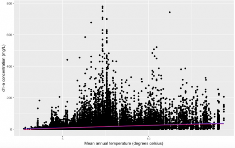
Figure 1. The relationship between regional mean annual water temperature and phytoplankton biomass in 17 states region in the U.S. Data from LAGOS-NE database (n= 65434). Phytoplankton population abundance is represented by chlorophyll-a concentration (mg/L). The temperature was measured on the hydrological unit scale (approximately 40 square miles in size). The blue line represents linear regression, and the red line represents quadratic regression.
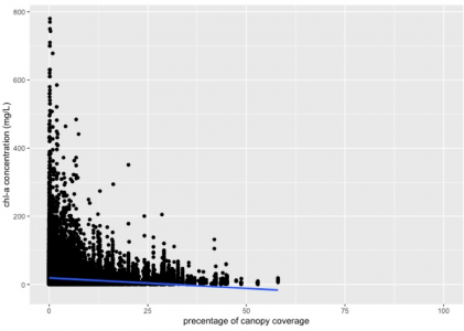
Figure 2. The relationship between canopy coverage and phytoplankton biomass in 17 states region in the U.S. Data from LAGOS-NE database (n=65434, R^2= 0.02677, p-value<2.2e-16). Phytoplankton population abundance is represented by chlorophyll-a concentration (mg/L).
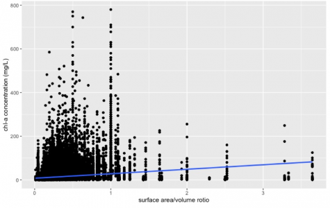
Figure 3. The relationship between lake size and phytoplankton biomass in 17 states region in the U.S. Data from LAGOS-NE database (n= 65434, R^2= 0.03756, p-value<2.2e-16). Phytoplankton population abundance is represented by chlorophyll-a concentration (mg/L), lake size is represented by the surface-to-volume ratio.
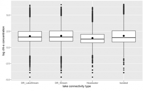
Figure 4. The relationship between lake connection type and phytoplankton biomass in 17 states region in the U.S. Data from LAGOS-NE database (n= 65434, F =154.6, p< 2e-16). “DR_LakeStream” represents streams that enter a lake and it has more lakes upstream. “DR_Stream” represents drainage streams that enter a lake. “Headwater” represents lakes that have no inflow stream but connect to downstream. “Isolated” represents lakes that have no inflow or outflow. Phytoplankton population biomass is represented by log-transformed chlorophyll-a concentration (mg/L).
The change in mean annual temperature can lead to a significant change in phytoplankton biomass as hypothesized (p-value<2.2e-16). There was a possible temperature tolerance range (0 °C to 16 °C) in Figure 1 since no observation can be found outside this range. The linear regression model (the blue line) suggested that within this range, there was a positive correlation between temperature and phytoplankton biomass (slope = 3.20419). And the quadratic model (the red line) suggested the same. The ANOVA test result showed that the linear model was a better fit to describe the relationship, and the difference in AIC scores of the two models is 44 (AICLinear=636336, AICQuadratic=636292).
Based on Figure 2, we can see that canopy coverage percentage can also significantly influence phytoplankton biomass (p-value<2.2e-16), and the linear regression model suggested a negative relationship between them (slope= -0.61429). This result supported the hypothesis. In addition, we can also notice that the chlorophyll-a concentration approximated zero when the canopy coverage is higher than 50%, whereas the highest value showed when canopy coverage is approximately 0%.
From Figure 3, the lake size also had a substantial influence on phytoplankton biomass (p-value<2.2e-16). A positive correlation between the surface-to-volume ratio and chlorophyll-a concentration can be observed from the graph, which corresponds with the prediction. Moreover, we can see most of the points were skewed and distributed in the bottom left corner of the figure, suggesting most of the observations were taken from deep lakes or streams (surface-to-volume ratio<1). But the positive slope of the linear model suggested that phytoplankton biomass increases in shallower water bodies.
According to Figure 4, chlorophyll-a concentration showed significant variance among different types of water body connections (F =154.6, p< 2e-16). A post hoc Tukey test showed that each group was significantly different from the other three groups, in particular, the isolated lake group showed the greatest distinction (about 10.227 in mean) from headwater lakes.
The results above suggested that phytoplankton can respond to temperature, irradiance, growing space, and water bodies connectivity change. This result increased the potential to use phytoplankton as a bioindicator in the water quality tests.
Discussion
The result indicates that increased temperature results in positive influences in chlorophyll-a concentration as predicted (Figure 1). Although only a small amount (3.8%) of observations can be well-explained by the linear model, the increase in p-value is still substantial and it is sufficient to conclude that temperature and phytoplankton abundance is positively correlated. This trend has also been observed in a similar study in Narragansett Bay, Rhode Island (Karentz & Smayda, 1984). Based on their analysis of 22 years of data (1959-1980), they found the succession of phytoplankton is primarily determined by temperature. Based on the analysis of the annual pattern of phytoplankton distribution, they also found that phytoplankton’s occurrence can be related to seasonality, where temperature played an important role. Phytoplankton species tend to reach their maximum growth rate when the water temperature is ranging from 7°C to 23°C, which is somewhat in agreement with this study. In this study, we can see a very similar abundance pattern of phytoplankton species which blooms in a temperature range from 7°C to 12°C. Low temperature limits the growth of phytoplankton by limiting their nutrient intake (Thomas et.al., 2017), which explains the low abundance of phytoplankton in cold water. However, we can also observe a chlorophyll-a concentration decline when the temperature is higher than 12°C. One possible reason for this result is that warming of the water can indirectly influence phytoplankton population size via increased grazing pressure (Lewandowska & Sommer, 2010). Warm temperature promotes zooplankton activity, just as it can promote phytoplankton activity. Giving that, in the long term, phytoplankton species tend to shrink their cell size to avoid herbivory (Lewandowska & Sommer, 2010). Thus chlorophyll-a concentration will also decline due to a reduced amount of chloroplast.
On the other hand, this water temperature analysis is limited and highly influenced by seasonality. The annual temperature studied here may not be enough to demonstrate the influence of seasonal changes in water temperature. And global warming events also had a profound effect on water temperature in recent years. The average value of the annual temperature records failed to show the variation caused by a gradual increase in temperature.
The result suggested that high canopy coverage over the lake resulted in a negative effect on phytoplankton growth. This trend is reasonable because sunlight is one of the decisive factors in the process of photosynthesis. Similar results can be found in a mesocosm study in the Baltic Sea (Sommer & Lengfellner, 2008), experiments in boreal lakes in ELA (Experimental Lake Area) (Findlay et.al.,2001) and observations from Lake Müggelsee, Berlin (Nicklisch, Shatwell & Köhler, 2008). Thus, the result supported the hypothesis that sunlight promotes the growth of phytoplankton. Also, Kojima (2000) found that phytoplankton biomass will experience a very significant reduction when the shaded water surface area was over 60%. The result of this study also suggested the same. In addition, Nicklisch, Shatwell, and Köhler (2008) also found that photoperiods have more influence than light intensity. The length of daytime is related to seasonality. Changes in seasons also lead to a change in water temperature. Thus, the influence of sunlight can be found to have a strong association with temperature influences.
Moreover, another study in North Sunter Reservoir, Jakarta (Juliastutie, Rinanti & Hendrawan, 2018) suggested that phytoplankton responses to sunlight were related to nutrient conditions, as it plays an important role in photosynthesis. In this case, the canopy coverage percentage data could also bring uncertainty to the result, since high canopy coverage also means high input of leaf litter in the freshwater ecosystem (Webster & Benfield, 1986). Such inputs often regulate community productivity by generating more primary and secondary production (Polis et. al., 1997), and leads to an increase in the phytoplankton biomass. Although we cannot see this increase in this study, the effect of forest litter is still going to influence the result. In this case, the conclusions related to sunlight were tentative.
Phytoplankton abundance was positively affected by the lake surface-to-volume ratio. This ratio indicates whether the lake is deep or shallow. The surface-area-to-volume ratio influences the uptake of light and nutrient and gas exchange of the lake. The higher the ratio, the shallower the lake or larger the surface area, which suggests the wider the region can contact the atmosphere. Also, we can see phytoplankton tended to favour shallow regions of a lake as the trend was going up in Figure 3. This is because deep mixing suppresses phytoplankton production due to light limitation (Diehl et. al., 2002). And because the internal loading of nutrients from sediments into the water column is generally much higher in shallow lakes than in deep lakes (Wetzel, 2001). In addition, a study based on observations from 540 lakes across the United States found that phytoplankton diversity also increased with the lake area (Stomp et.al.,2011). This finding resembles the common type of species-space relationship in many different ecosystems. According to the theory of island biogeography (MacArthur and Wilson, 1967), larger ecosystems are likely to have more species due to higher immigration rates and lower extinction. In other words, large ecosystems have more resources and higher carrying capacity, which lowers inter- and intra-species competitions. The lakes in 17 states in the U.S. can be considered as “islands” in terrestrial environments. Therefore, this theory can be applied to explain the result of this study. Also, the positive species-area relationship can be observed in other studies as well, Reche et.al. (2005) and Smith et.al. (2005) founded that this positive correlation also exists in a variety of habitats from salt marshes to alpine lakes, and experimental microcosms to oceans.
According to Figure 4 and Tukey’s test result, there was a significant influence of lake connection on phytoplankton biomass. This result supported the hypothesis as expected. Hydraulic interventions that decreased the discharge and/or flow velocity together with increased nutrient loads led to eutrophication in freshwater ecosystems (Sabater et al., 2008). Planktons are exposed to continuous washout during their growth period and transportation. Thus, a special area in the freshwater system with a slow current and large storage can be important for the persistence of planktonic populations. This area must fulfill two criteria (Reynolds & Descy, 1996). First, this area must be flushed by water flow at a sufficient rate to continuously take away the newly produced biomass. Second, the water flow in this area must be isolated from the rapid main flow to create a relatively undisturbed environment for phytoplankton to grow. In this case, a lentic system with low water turbulence can stratify these requirements. And isolated lake systems can provide more of this kind of area. However, such special areas for phytoplankton growth can also be found within each different connectivity type of lakes/streams. For example, a depositional area behind the stream boulder can be a suitable place for phytoplankton to grow. This suggests that the physical characteristics related to water current can be also considered on a smaller scale, such as in pool-riffle scale or microhabitat scale. Moreover, Istvánovics et.al.(2010) suggested that in both the lotic and lentic systems, physical forcing (water current) will act together with nutrient limitation to regulate the phytoplankton population. This also can be one of the limitations of the result.
In this study, only the spatial differences of environments were discussed, but temporal changes in the environment are also worth analyzing. Some studies have accessed and compared their historical data and then discovered that water quality has declined in recent years (Suthers, Rissik, & Richardson, 2019). Recent climate change and rapid urbanization added more pressure to the survival of all freshwater organisms. Climate affects phytoplankton indirectly by changing resource availability, mainly nutrients and light (Winder & Sommer, 2012). Warming spring water temperature also changes the timing and magnitude of phytoplankton blooms (Townsend et.al.,1994). Urbanization caused a 50% variation in phytoplankton biomass in a 23-year period due to land reclamation and pollutions (Wang et al.,2020). Based on these findings, historical limnological data from LAGOS-NE is worth exploring in future studies since they are likely to provide resemblant results. Consequently, further proving that phytoplankton can be a bioindicator of water quality.
The result of this study suggested that phytoplankton is qualified as a bioindicator of water quality since it is sensible enough to detect and respond to abiotic changes including temperature, sunlight, lake size, and lake connectivity. Although all the abiotic factors listed have been found to have an association with N and P conditions in the water, the performance of phytoplankton is still good enough to reflect the difference. Identifying the biomass of the phytoplankton group and relating it to the water quality parameters can help to understand the ecological dynamics of the freshwater system. The operation and maintenance tasks are necessary since water quality directly influences the living environment for all aquatic organisms. Moreover, this application can also be used in marine environments. Studies have found that in the marine ecosystem, phytoplankton’s biomass, distribution, and diversity can respond to wastewater pollutant (Webber et.al.,2005), industrial pollutant (Shekhar et.al.,2008), trophic state changes (Coelho, Gamito & Pérez-Ruzafa, 2007), and even hurricane impacts (Peierls, Christian& Paerl, 2003). All the evidence shows the phytoplankton’s great potential as an effective and efficient water quality indicator.
Reference:
Amengual-Morro, C., Niell, G. M., & Martínez-Taberner, A. (2012). Phytoplankton as bioindicator for waste stabilization ponds. Journal of Environmental Management, 95, S71-S76.
American Public Health Association, American Water Works Association, Water Pollution Control Federation, & Water Environment Federation. (1915). Standard methods for the examination of water and wastewater (Vol. 2). American Public Health Association.
Behrenfeld, M. J. (2001). Biospheric primary production during an ENSO transition. Science (American Association for the Advancement of Science), 291(5513), 2594-2597.
Bellinger, E. G., & Sigee, D. C. (2015). Freshwater algae: identification, enumeration and use as bioindicators. John Wiley & Sons.
Boyer, J. N., Kelble, C. R., Ortner, P. B., & Rudnick, D. T. (2009). Phytoplankton bloom status: Chlorophyll a biomass as an indicator of water quality condition in the southern estuaries of Florida, USA. Ecological indicators, 9(6), S56-S67.
Coelho, S., Gamito, S., & Pérez-Ruzafa, A. (2007). Trophic state of Foz de Almargem coastal lagoon (Algarve, South Portugal) based on the water quality and the phytoplankton community. Estuarine, Coastal and Shelf Science, 71(1-2), 218-231.
Diersing, N., & Nancy, F. (2009). Water quality: Frequently asked questions. Florida Brooks National Marine Sanctuary, Key West, FL.
Findlay, D. L., Kasian, S. E. M., Stainton, M. P., Beaty, K., & Lyng, M. (2001). Climatic influences on algal populations of boreal forest lakes in the Experimental Lakes Area. Limnology and Oceanography, 46(7), 1784-1793.
Gordon, H. R., & McCluney, W. R. (1975). Estimation of the depth of sunlight penetration in the sea for remote sensing. Applied optics, 14(2), 413-416.
Istvánovics, V., Honti, M., Vörös, L., & Kozma, Z. (2010). Phytoplankton dynamics in relation to connectivity, flow dynamics and resource availability—the case of a large, lowland river, the Hungarian Tisza. Hydrobiologia, 637(1), 121-141.
Juliastutie, C., Rinanti, A., & Hendrawan, D. (2018). Correlation of physics and chemical factors on phytoplankton distribution pattern in North Sunter Reservoir, Jakarta. In MATEC Web of Conferences (Vol. 197, p. 13014). EDP Sciences.
Karentz, D., & Smayda, T. J. (1984). Temperature and seasonal occurrence patterns of 30 dominant phytoplankton species in Narragansett Bay over a 22-year period (1959–1980). Mar. Ecol. Prog. Ser, 18, 277-293.
Kojima, S. (2000). Corroborating study on algal control by partial shading of lake surface. Raw Waste Water, 42(5), 5-12.
Kunz, T. J., & Diehl, S. (2003). Phytoplankton, light and nutrients along a gradient of mixing depth: a field test of producer‐resource theory. Freshwater Biology, 48(6), 1050-1063.
Leibold, M. A. (1989). Resource edibility and the effects of predators and productivity on the outcome of trophic interactions. The American Naturalist, 134(6), 922-949.
Lewandowska, A., & Sommer, U. (2010). Climate change and the spring bloom: a mesocosm study on the influence of light and temperature on phytoplankton and mesozooplankton. Marine Ecology Progress Series, 405, 101-111.
MacArthur, R. H., & Wilson, E. O. (2001). The theory of island biogeography (Vol. 1). Princeton university press.
Moses, S. A., Janaki, L., Joseph, S., Justus, J., & Vimala, S. R. (2011). Influence of lake morphology on water quality. Environmental monitoring and assessment, 182(1-4), 443-454.
Nicklisch, A., Shatwell, T., & Köhler, J. (2008). Analysis and modelling of the interactive effects of temperature and light on phytoplankton growth and relevance for the spring bloom. Journal of Plankton Research, 30(1), 75-91.
Parmar, T. K., Rawtani, D., & Agrawal, Y. K. (2016). Bioindicators: the natural indicator of environmental pollution. Frontiers in life science, 9(2), 110-118.
Peierls, B. L., Christian, R. R., & Paerl, H. W. (2003). Water quality and phytoplankton as indicators of hurricane impacts on a large estuarine ecosystem. Estuaries, 26(5), 1329-1343.
Polis, G. A., Anderson, W. B., & Holt, R. D. (1997). Toward an integration of landscape and food web ecology: the dynamics of spatially subsidized food webs. Annual review of ecology and systematics, 28(1), 289-316.
Reche, I., Pulido-Villena, E., Morales-Baquero, R., & Casamayor, E. O. (2005). Does ecosystem size determine aquatic bacterial richness?. Ecology, 86(7), 1715-1722.
Reynolds, C. S., & Descy, J. P. (1996). The production, biomass and structure of phytoplankton in large rivers. Large Rivers, 161-187.
Sabater, S., Artigas, J., Durán, C., Pardos, M., Romaní, A. M., Tornés, E., & Ylla, I. (2008). Longitudinal development of chlorophyll and phytoplankton assemblages in a regulated large river (the Ebro River). Science of the total environment, 404(1), 196-206.
Sarnelle, O. (1992). Nutrient enrichment and grazer effects on phytoplankton in lakes. Ecology, 73(2), 551-560.
Shekhar, T. S., Kiran, B. R., Puttaiah, E. T., Shivaraj, Y., & Mahadevan, K. M. (2008). Phytoplankton as index of water quality with reference to industrial pollution. Journal of Environmental Biology, 29(2), 233.
Smith, V. H., Foster, B. L., Grover, J. P., Holt, R. D., Leibold, M. A., & deNoyelles, F. (2005). Phytoplankton species richness scales consistently from laboratory microcosms to the world's oceans. Proceedings of the National Academy of Sciences, 102(12), 4393-4396.
Sommer, U., & Lengfellner, K. (2008). Climate change and the timing, magnitude, and composition of the phytoplankton spring bloom. Global Change Biology, 14(6), 1199-1208.
Soranno P., Cheruvelil, K., (2017) LAGOS-NE-GEO v1.05: A module for LAGOS-NE, a multi-scaled geospatial and temporal database of lake ecological context and water quality for thousands of U.S. Lakes: 1925-2013. Environmental Data Initiative.
Soranno P., Cheruvelil, K., (2019) LAGOS-NE-LIMNO v1.087.3: A module for LAGOS-NE, a multi-scaled geospatial and temporal database of lake ecological context and water quality for thousands of U.S. Lakes: 1925-2013. Environmental Data Initiative.
Soranno, P. A., Bacon, L. C., Beauchene, M., Bednar, K. E., Bissell, E. G., Boudreau, C. K., ... & Cheruvelil, K. S. (2017). LAGOS-NE: a multi-scaled geospatial and temporal database of lake ecological context and water quality for thousands of US lakes. GigaScience, 6(12), gix101.
Soranno, P. A., Bacon, L. C., Beauchene, M., Bednar, K. E., Bissell, E. G., Boudreau, C. K., ... & Cheruvelil, K. S. (2017). LAGOS-NE-LOCUS v1.01: A module for LAGOS-NE, a multi-scaled geospatial and temporal database of lake ecological context and water quality for thousands of U.S. Lakes: 1925-2013. Environmental Data Initiative.
Soranno, P. A., Lottig, N. R., Delany, A. D., & Cheruvelil, K. S. (2019). LAGOS-NE-LIMNO v1. 087.3: A module for LAGOS-NE, a multi-scaled geospatial and temporal database of lake ecological context and water quality for thousands of US Lakes: 1925-2013.
Steele, J. H. (1962). Environmental control of photosynthesis in the sea. Limnology and oceanography, 7(2), 137-150.
Stomp, M., Huisman, J., Mittelbach, G. G., Litchman, E., & Klausmeier, C. A. (2011). Large‐scale biodiversity patterns in freshwater phytoplankton. Ecology, 92(11), 2096-2107.
Suthers, I., Rissik, D., & Richardson, A. (Eds.). (2019). Plankton: A guide to their ecology and monitoring for water quality. CSIRO publishing.
Tait, L. W., & Schiel, D. R. (2013). Impacts of temperature on primary productivity and respiration in naturally structured macroalgal assemblages. PLoS One, 8(9), e74413.
Thomas, M. K., Aranguren‐Gassis, M., Kremer, C. T., Gould, M. R., Anderson, K., Klausmeier, C. A., & Litchman, E. (2017). Temperature–nutrient interactions exacerbate sensitivity to warming in phytoplankton. Global Change Biology, 23(8), 3269-3280.
Townsend, D. W., Cammen, L. M., Holligan, P. M., Campbell, D. E., & Pettigrew, N. R. (1994). Causes and consequences of variability in the timing of spring phytoplankton blooms. Deep Sea Research Part I: Oceanographic Research Papers, 41(5-6), 747-765.
US Geological Survey, US Department of Agriculture, & Natural Resources Conservation Service. (2011). Federal Standards and Procedures for the National Watershed Boundary Dataset (WBD).
Wang, R., Wu, J., Yiu, K. F., Shen, P., & Lam, P. K. (2020). Long-term variation in phytoplankton assemblages during urbanization: A comparative case study of Deep Bay and Mirs Bay, Hong Kong, China. Science of the Total Environment, 745, 140993.
Webber, M., Edwards-Myers, E., Campbell, C., & Webber, D. (2005). Phytoplankton and zooplankton as indicators of water quality in Discovery Bay, Jamaica. Hydrobiologia, 545(1), 177-193.
Webster, J. R., & Benfield, E. F. (1986). Vascular plant breakdown in freshwater ecosystems. Annual review of ecology and systematics, 17(1), 567-594.
Winder, M., & Sommer, U. (2012). Phytoplankton response to a changing climate. Hydrobiologia, 698(1), 5-16.
Learning Significance